Gas Laws

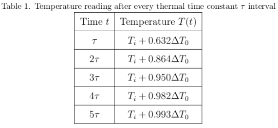
The behavior of gases can be modeled by using the concept of an ideal gas. An ideal gas is a gas made up of particles that 1) are infinitesimally small such that the individual particles do not occupy a volume (point particles), 2) only collide elastically, 3) have motions that are independent, i.e., no intermolecular forces manifest between the particles. While such a gas is only a theoretical concept, gases can be approximated to be ideal under certain conditions. For example, by making the container of the gas large, the point particle model of the gas particles becomes more valid.

One can describe the properties of a gas without referring to its microscopic particles. This is through the emergent properties of these particles that can be measured by analyzing the gas as macroscopic entity. Such properties include pressure P, volume V, and temperature T. These properties indicate the state of a gas, and an equation relating these properties is called an equation of state. An equation of state is of great significance because it allows for some of the properties to be calculated instead of measuring it directly. It also implies that an ideal gas cannot have an arbitrary set of values for these properties. That is, for every given ideal gas consisting of N particles, the ordered array Z=(P, V, T) is a unique array of numbers describing its state.

One equation of state is the ideal gas law which assumes an ideal gas

PV=NkT

(1)

where k is the Boltzmann constant with a value of 1.3806488 x 10^-23 m^2•kg•s^-2•K^-1. When certain properties are made constant, one can easily derive the following relationships:

PV=K

(2)

V/T=C

(3)

where K=NkT and  C=Nk/P. When temperature is made constant, K is constant and (2) shows the inverse proportionality of pressure and volume. This is known as Boyle’s Law. Meanwhile, under the conditions where the pressure is constant (which is approximately the case in our usual environment), (3) shows that volume is directly proportional to temperature. This is known as Charles’ Law. In this experiments, relations (2) and (3) are verified.

I. Boyle’s Law

A gas carrying-container consisting of two compartments A and B (refer to Figure 1) is subjected to varying pressure by placing different masses on top of the piston in compartment A. Temperature is made constant by immersing compartment B in boiling water where the temperature is unvarying. For each mass 100 g, 150 g, 200 g, 250 g, the pressure and the corresponding volume of compartment A is measured.

Figure 1. Simplified model of the setup for Boyle’s law. Compartment B is immersed in boiling water.

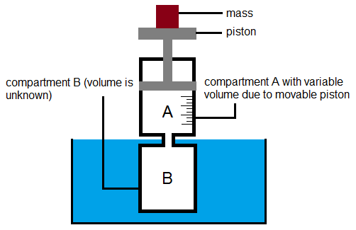
In the actual experiment, compartment B has a much more complicated geometry and thus its volume is unknown. Compartment A is a graduated cylinder and its volume is measurable given its diameter. When the piston is empty, compartments A and B is filled with gas. Noting that the volume of the gas in the container is V=V(A)+V(B) and that V(B) is constant, then from (2)

V=K/P

V(A)+V(B)=K/P

V(A)=K(1/P)-V(B)

(4)

Plotting the volume of A versus the reciprocal of pressure gives a linear curve where the slope is K and the negative of the y-intercept is the volume of B. When the temperature is known, the number of particles N can be calculated since K=NkT.

Figure 2. Graph of volume of A versus reciprocal of pressure.

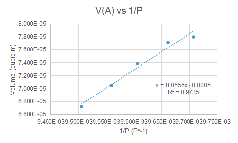
From the data in Figure 2, the calculated volume of B is 500 mL and N=10^19 particles.

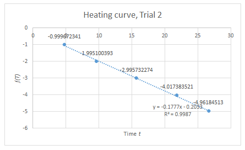
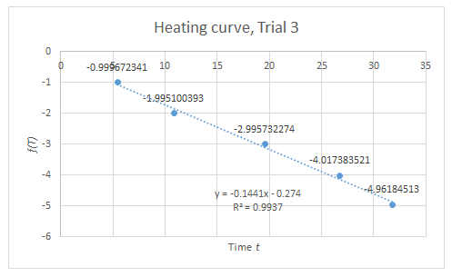
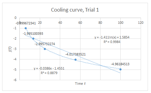
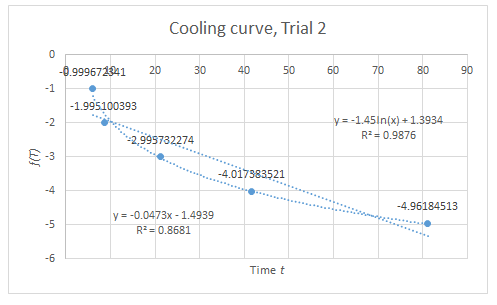
II. Charles’ Law

The setup for this part is only a modification of the setup for Boyle’s Law. The apparatus must be subjected to varying temperature. Thus, instead of boiling water, an initially hot volume of water is used, and chunks of ice are added to vary the temperature. At equal intervals of time, the temperature and the corresponding height of the piston are measured. Through a similar approach in the derivation of (4), the relation of volume A and temperature at any given time is

V(A)=CT-V(B)

(5)

Plotting the volume of A versus the temperature gives a linear curve where the slope is C. When the pressure is known, the number of particles N can be calculated since C=Nk/P.

Figure 3. Graph of volume of A versus temperature.

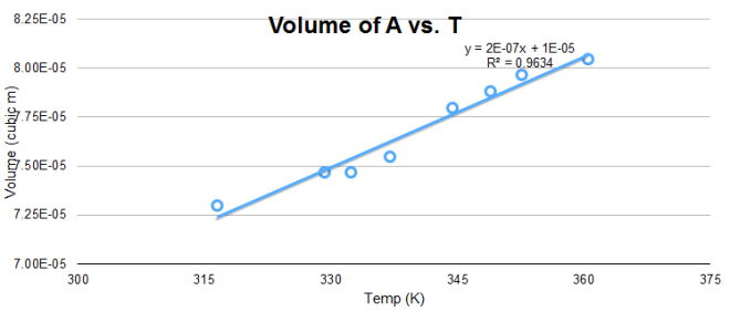
From the data in Figure 3, the calculated N is 10^19 particles, similar to the previous calculation. However, discrepancy arises on the value of the y-intercept since it is expected to be a negative number.

From the R^2 values of the graphs, the trend dictated by (2) and (3) are verified, but only to some extent since these values are not sufficiently close to unity. However, considering the various sources of systematic error, the data suggest that if these error sources were minimized, a more linear trend can be expected.

There are several sources of systematic error for this experiment; the following are only some: First, gas leaks on the container. In the Boyle’s Law setup, when a mass is removed from the piston, it is expected that the piston goes back to its initial height. However, this does not happen. Instead, the piston remains on its position as if the mass is still on top of it. This implies the possibility of gas leak. Second, it takes time for the piston to reach its “equilibrium height” (height where the piston is already static). Thus, it is up to the judgement of the experimenter to determine if the piston is already in steady-state. This source of error has a much significant effect in the Charles’ Law setup. It is assumed in the experiment that at every instant where the temperature is recorded, the piston is already at its corresponding steady-state height. However, if it the piston lags behind too much to reach its steady-state, this assumption becomes invalid. This can account to the much lower R^2 value of the graph in Charles’ Law. Lastly, friction between the piston and the wall of the container can hinder the piston to reach its supposed equilibrium height.

 

Calorimetry

Heat is the energy transferred between two bodies that causes a change in temperature. The amount of heat q needed for a body to change its temperature by some value ΔT is dependent on its composition and mass. The heat capacity C accounts for this thermodynamic property due to the body’s mass and composition. For a body of a certain mass and composition, the heat capacity C is the amount of heat q needed to change the temperature by one Kelvin unit:

q=CΔT

(1)

The value of the heat capacity is dependent on the mass and the composition of the body. It turns out that this value is also proportional to the mass m of the body. Thus,

C=mc

(2)

q=mcΔT

(3)

where c is a constant for a body of given composition. This constant is the specific heat capacity, and it accounts for the dependence of q on the body’s composition.

In an adiabatic system, heat cannot enter or leave the system. Suppose the system is composed of n bodies, then

q1+q2+…+qn=0

(4)

A calorimeter is a device that is used to determine the specific heat capacities of materials. The calorimeter and everything inside it is assumed to be a closed system where matter and heat is conserved. The conservation of these quantities in the system are utilized to compute the specific heat of a material.

In this experiment, the specific heat of metals (copper and aluminum) are measured. The calorimeter (cal) used is a coffee cup. Inside it is a certain volume of water and the metal (m). Thus,

q(cal)+q(w)+q(m)=0

q(m)=-[q+C(cal)ΔT]

(5)

The heat capacity of the calorimeter is still unknown, and this must be measured first to measure the specific heat of the metals. This process is termed as the calibration of the calorimeter.

We first replace the metal with a hot water (w’). We assume that the initial temperatures T(0) of the calorimeter and the water inside it  are equal as the two bodies are in thermodynamic equilibrium. When (w’) is mixed with inside the calorimeter, the three bodies will progress towards a new equilibrium temperature. Consequently, (w’) loses heat. This lost heat must be gained by (cal) and since the system is closed:

q(cal)>0, q(w)>0, q(w’)<0

-q(m)=q(cal)+ q

(6)

Since the specific heat capacity of water is known (1 calorie or 4.184 kJ/K•m), C(cal) can be computed by rewriting (6) into

(7)

The expression of C(cal) is dependent on the equilibrium temperature of the system Tf. When, this value is known, C(cal) can readily be calculated through (7) and (3).

Taking the time of complete mixture of and (w’) as t=0, the temperature of the system T is taken every 30 seconds for 5 minutes using a thermocouple. The graph of ln(T) vs. t will be linear (this is intuitive considering the discussion on “Temperature Measurement”). The y-intercept of this graph b gives the final temperature by

Tf=exp(b)

(8)

Three calibration trials are done. The value taken to be C(cal) is the average of the three values.

Figures 1-3. Calibration curve for Trials 1-3, respectively.

Tables 1-3. Calibration data.

The average of the three values for C(cal) is 37.66 kJ/K. Note however that the average value has a high relative deviation.

With the heat capacity of the calorimeter known, the specific heat of the metals can now be measured. Returning to (6), this can be written as

(9)

The method of measurement and computation is very similar to the calibration. In this part however, it is the metal that is being investigated instead of the calorimeter. Only one trial is done for the measurement of the specific heat of each metal.

Tables 4-5. Data for the measurement of the specific heat capacity of Al and Cu.

The literature value of the specific heat capacity of aluminum and copper is 0.900 kJ/m•K and 0.386 kJ/m•K, respectively [1]. The relative deviation of the measured value from the literature value is 12% for aluminum and 1% for copper. This means that for equal masses, a copper metal is more sensitive to temperature changes than an aluminum metal.

The sources of error for this experiment arise mostly from the approximation that the system is ideally closed. For example, in getting the equilibrium temperature of the system, one must wait a sufficient duration of time for the system to reach thermodynamic equilibrium. However, one must not wait too long, for the heat loss of the calorimeter system might become too significant for the adiabatic approximation to not hold.

Temperature measurement

While temperature in everyday language is associated with the hotness and coldness of a body, formally (but not complete) it is a value related to the average kinetic energy of the molecules of a given body. When two bodies A and B of different temperatures are brought in contact, after some time, both A and B will be at the same temperature and it is said that A and B are in thermal equilibrium. This tendency of matter to progress towards thermal equilibrium is the main principle of thermometers. When reading the temperature of a body, the body and the thermometer are brought in contact. After a sufficient duration of time, thermal equilibrium is reached. Thus, at this state, knowing the temperature of the thermometer will give the temperature of the body as well. This is done efficiently if the thermometer do not cause significant changes in the temperature of the body (e.g. small mass of thermometer). Thermometers have measurable properties that are dependent on temperature. The changes in these properties give an indirect way of measuring the temperature.

When a thermometer is brought in contact with a body, its temperature does not jump instantly to the equilibrium reading. The temperature change is more of a continuous curve. Consider a thermometer at an instantaneous temperature T(t) and where its equilibrium temperature (final reading) is Tf. As time goes by, T(t) approaches Tf, i.e., the difference between Tf and T(t) decreases. Let this difference be ΔT (note that this value is a function of time t). The instantaneous rate of change of ΔT for some common thermometers is practically proportional to ΔT at that instant of time, i.e.,

(1)

where k is a positive constant. The negative sign accounts for the fact that ΔT decreases as time increases. Solving this first order differential equation and noting that ΔT=Tf-T(t), we arrive at

(2)

where τ is the thermal time constant τ=1/k, and Ti is the initial temperature of the thermometer (see Proof). Equation (2) provides the trend of the temperature of a thermometer as it approaches thermal equilibrium. Note that it takes an infinite amount of time to reach Tf. However, at sufficiently large t, not only that the exponential function is approximately zero, but its value changes very little (its derivative). Thus, at a sufficiently large t, the temperature reading T(t) is almost unvarying and approximately equal to Tf.

In this experiment, the temperature curve of a thermometer being heated and cooled is analyzed and this curve is verified if it follows the trend of the model (2).

In setting the initial temperature of the thermometer, it is dipped in ice-cold water and boiling water for the heating and cooling setup, respectively. When the reading remains constant, the temperature is taken to be Ti, and the thermometer is dipped in boiling water and ice-cold water for the heating and cooling setup, respectively. This instant is taken to be t=0. As the thermometer is allowed to reach thermal equilibrium, certain temperature readings are noted of their time of occurrence. The noted temperatures are the expected readings at certain values of t that is a multiple of τ.

Equation (2) can be easily shown to be equivalent to

(3)

Let the left-hand side of (3) be f(T). Then, the graph of f(T) versus t is linear. The slope m of this linear graph gives the value of τ

(4)

For the heating setup, the data is summarized by the following graphs.

Figures 1-3. Heating curves.

It is evident from the graphs, with R^2≈1, that the heating setup follows very well the trend predicted by (3). The best estimate value for the thermal time constant is 6.252±0.688 1/s.

For the cooling setup, the data is summarized by the following graphs.

Figures 3-6. Cooling curves. The equation at the upper right side is the fitted logarithmic curve; the equation at the lower left side is the fitted linear curve. Note the R^2 of linear curves are not sufficiently close to unity.

Contrary to the predicted trend, the graph of f(T) versus t is not linear. Instead, a logarithmic curve fits better than a linear curve for all three trials. This implies that in this setup, the relation of T(t) to t is described better by the following equation (see Proof):

(5)

where κ is the coefficient of the logarithmic function in the equations on Figures 3-6.

If however the linear curve is considered despite the low values of R^2, the best estimate for the thermal time constant is 23.93±2.79 1/s (compare this to this to the other value 6.252±0.688 1/s). If the model holds for both setups, the value of τ from both setups must be equal, since the same thermometer is used and τ is a property of a body.

Sources of error include, but is not limited to, reaction time of experimenter in noting the time of temperature occurrence and the approximation that all systems are ideal.

Appendix

Proof for (1):

QED.

Proof for (5):

 QED.

References:

1. NIP Physics lab manual.
2. University Physics, 13th ed.

This has nothing to do with Physics 103.1 but it’s fun nonetheless

Consider the following animation:

Source: http://9gag.com/gag/anNebZB

In the animation, it is evident that the motion of a particle oscillating about the origin at any arbitrary but constant direction is equivalent to an orbital motion about a point which in turn orbits the origin. We wish to find a mathematical expression that shows this equivalence. It is easier to define the motion of the particle at first as the latter (orbital). The task now is to show that this equation can be written in a form that explicitly describes a motion of the former type (oscillatory).

I. Orbital Motion

Consider the following figure.

Figure 1. A circle (blue) of radius r centered at C revolves about the origin. A particle (red dot) also revolves at the center of this moving circle at a distance r away.

The circle of radius r revolves around the origin such that the origin is always on the circle. Thus, the center C is also of distance r away from the origin. The motion of C with respect to the origin as a function of time t is described by the vector

(1)

where ω1 is the angular speed of C, and Φ1 is the phase which accounts for the initial position of C (in the animation, the center is initially at the +y-axis and Φ1=π/2) . We then consider any point on the circle as a particle that moves (this corresponds to the dots in the animation). The circle is rotating and therefore the particles revolve around the center with some angular speed ω2. The position of an arbitrary particle with respect to the center of the circle C is

(2)

(for the red particle in the animation,  Φ2=π/2). The position of the particle with respect to the origin at any given time is just the sum of these two vectors. Using trigonometric identities,  the position vector of any particle can be written as

(3)

II. Oscillatory Motion

With respect to the origin, the motion of any particle is confined on a unique line passing through the origin. This is very evident on the red particle in the animation as it only oscillates along the y-axis. Specifically, while the distance of the particle from the origin (norm of R) varies over time, its position vector R is always parallel to some constant unit vector u. In other words, when R is not the zero vector the unit directional vector of R can only change in sign:

(4)*

Figure 2. A particle’s motion is confined on a line passing through the origin.

A motion of this type takes the following form (see Proof):

(5)

where f(t) is the variable norm of the position vector and u is a constant unit vector. Thus, the motion of the particles in the animation can both take the form of (3) and (5).

The form of (3) is already similar to (5). The vector part of (3) is a unit vector and is therefore the u in (5); the remaining part is the norm f(t):

(6)

(7)

However, we know that u is constant with respect to time. Equation (7) is thus true if and only if

(8)

so that the right-hand side of (7) is no longer a function of time. Relation (8) is reasonable since, in the animation, the circle is revolving clockwise while the particles are revolving around the center counterclockwise.

Let ω=ω1. Applying (8) to (3), we arrive at

(9)

which is finally the equation describing the motion of the particles in the animation. Equation (9) shows that the complex orbital motion of the particles is indeed equivalent to a simple sinusoidal oscillation along a fixed and unique axis defined by u. Note also that the amplitude is indeed twice the radius of the revolving circle.

In the case of that in the animation, Φ1=π/2, and the value of Φ2 will depend on what particle is being observed. For the red particle (for all instances), Φ2=π/2. For the green particle on the first circle (consisting of two particles only), Φ2=-π/2 (note that the value of Φ1 is not unique and is valid up to an additive constant that is a multiple of 2π).

It is interesting to investigate the motion of the particles on the first circle. For the red and green particles respectively, the corresponding vector-valued functions are

(10, 11)

The following equations shows that the red particle oscillates along the y-axis and the green particle along the x-axis. Also, whenever the red particle is at maximum displacement from the origin, the green particle is at the center (zero displacement) which is the case when t=0 (see animation).

III. Appendix

Proof for (5):

When f(t) is non-zero,

*Note that the or in (4) is an exclusive or. The disjunction in the fourth line of this proof is also exclusive since we restricted the value of f(t) to be non-zero.

Diffraction and Interference

I. Diffraction from a single slit

A laser beam is directed unto a narrow slit and a diffraction pattern is observed at a screen placed sufficiently far from the slit. Diffraction is observed in this setup due to the self-interference of the light beam. Recalling Huygen’s principle, every point of a wave front can be considered a light source. Waves from these point sources interfere with each other and form a diffraction pattern with bright and dark bands.

We consider the light wave coming to the slit as plane waves. As the plane wave arrives at the slit, secondary waves spread out in-phase. Assuming that the distance between the slit and the screen L is very large, the rays from every secondary wavelets can be considered to be parallel but converges at point P(x=∞, y). This is why L must be very large compared to the slit width a. The setup in-principle is shown below.

Figure 1. Slit with width a and a screen L (very large) distance away from the slit.

In the interest of locating the intensity minima (destructive interference), let P be a minima. Consider first dividing the slit in half such that given a point in the slit A(x=0, y≥0), there corresponds another point in the slit A'(x=0, y≤0) such that the distance between A and A’ is always a/2. For a particular pair (A ,A’)=(y=a/2, y=0) as shown in Figure 1, the path difference |r2-r1| must be m(λ/2), where m is an odd number, in order for the two waves to arrive at P completely out of phase. Since there exist a one-to-one correspondence (A, A’) that spans every point in the slit, the total sum of every wavelet in the slit is therefore zero at P, that is, if a is very small such that |r2-r1| for any given (A, A’) is conserved. Finally, we see that there is a minima at y if and only if

y = mλL/a

(1)

So far, the allowable values for n are odd integers. However, if the slit is divided into k parts (k=2 in the previous analysis), where k is an even number, there is also a one-to-one correspondence (A, A’) that spans every point in the slit where the the distance between A and A’ is conserved: dist(A, A’)=a/k. This gives to another set of minima. Thus, in (1) m can be any integer since k is always even. Negative integers corresponds to minima below y=0.

Knowing the values of the other variables (which are mostly lenghts), the wavelength of the light used can be determined using the setup.

For calculating the actual L which is strictly the length that light has traveled from the slit to the screen, the following method is applied:

Figure 2. Calculation for actual L. Slit and diffraction pattern is positioned at height h or h’.

The y value for the minima are determined by taking the width of the bright bands and dividing by 2 to get the distance from the center.

Figure 3. Experimental measurement of y.

Table 1 summarizes the data for this part of the experiment.

Table 1. Data for single slit diffraction.

The light source used is a red laser. The wavelength of red light lies at 650-750 nm [1]. For the 0.04 mm slit, the calculated average wavelength falls at the range while the wavelength from 0.02 mm slit is off by 18% from the upper bound of the range. One very significant source of error is deciding where the dark band is actually located at the pattern. The dark parts of the pattern are wider than expected. However, not all of these parts correspond to y. These are not points of completely destructive interference, but light intensity at these parts may only be actually very low. It is considered that the middle of the dark bands corresponds to y. But, locating the middle is often left to the decision of the experimenter and thus subjective. In fact, for m=1, a=0.02 mm every 1 mm measurement of y adds 36 nm to the wavelength calculation.

II. Interference from two slits:

A. Fringes

In this part, the same setup is applied but the configuration of the slit is changed: two slits are used instead of just one. Here, an interference pattern is observed on the screen located a distance L from the slits.

We invoke the same assumptions and approximations from the previous analysis in diffraction. Taking into account the interference alone of the waves from the two slits, we neglect the effects of diffraction. Thus, the slits are considered to be very narrow such that there is only one point in which a wavelet originate. The interference then is between the wavelets from each slit. The setup in-principle is shown in the figure below.

Figure 4. Interference from two slits. One wavelet per slit is considered. The interference pattern is due to the interference of the two point sources.

The pattern seen in the screen is due to the constructive and destructive interference of the waves. For a varying point in the screen P(x=L, y), the distance that the wavelets travel varies as well and the difference of these path lengths causes alternating bright and dark fringes to form. At a point where there is completely no light (minima), the waves arrive completely out of phase, i.e., |r2-r1|=(n+1/2)λ, where n is any integer. Meanwhile, at the brightest part of the bright fringes (maxima), the waves arrive in phase, i.e., |r2-r1|=nλ, where n is an integer. Finally, we see the following relations hold:

y = nλL/d

(2, intensity maxima)

y = (n+1/2)λL/d

(3, intensity minima)

We can also see that the Δy between two successive maxima and minima is λL/2d. Intuitively, the center of the bright fringes are the location of the maxima and the center of the dark fringes correspond to the minima. Then, the width w of the bright fringes is just twice the Δy

w = λL/d

(4)

Figure 5. Derivation of (4).

Alternatively, w can be measured approximately by measuring the width of the bright bands (by diffraction envelope) and dividing by the number of its bright fringes.

Table 2. Theoretical and experimental width of bright fringes.

From Table 2, to some extent the theoretical and experimental values for the width are consistent with each other. Errors arise mostly from the sensitivity of the setup (dealing with values in the magnitude of 10^(-3)) and deciding which fringes at the sides of a diffraction envelope belong to a band.

B. Calculating the slit width.

Equation (1) provides an expression for the slit width a. Using the setup for double slit interference and with a known value of the wavelength, a can be calculated.

The slit configuration is a=0.04 mm, d=0.25 mm. The labeled wavelength of the laser source was not noted, unfortunately. The average of the wavelength calculation in the single slit diffraction was used: 804 nm.

Table 3. Slit width calculation.

Table 3 shows high accuracy of the theoretically determined a compared to the labeled slit width. The equation used for the calculation of a is (1) which applies to a single slit. The high accuracy of data implies that the diffraction envelope pattern of the double slit setup still depends on the slit width a.

III. Appendix

Figure 6. General setup showing a single slit diffraction pattern.

Figure 7. Interference pattern of slit configuration: a=0.08 mm, d=0.25 mm. The first bright band of the diffraction envelope is divided by five fringes.

Figure 8. Interference pattern showing diffraction envelope and small fringes due to interference.

Reflection and refraction

I. Reflection

A ray of light was made to hit three types of mirrors: flat, convex, and concave. The mirror is positioned on the optical disk such that the line of symmetry of the curve coincides with the 0° ray of the optical disk, and the peak of curvature coincides with the origin. For all three cases, three incident angles are applied: 0°, 10°, and 20°. All nine cases lead to the same result: if the incident ray enters at the x° ray of one side of the optical disk, the reflected ray exits at the same ray but of the opposite side. This is exactly the law of reflection.

Fig. 1. Reflected ray at 10°. Red lines indicate incident rays; green lines indicate reflected rays.

However, what makes this experiment less trivial is that the same results apply whether the mirror used is flat or curved; it as if the ray, for all nine cases, hits only one type of mirror.

For the flat mirror, it is obvious that the normal line coincides with the 0° ray. But, the same is also true for the other mirrors with curved surfaces. The placement of the mirrors caused this unvarying result. Considering that the curve of the surface is smooth and continuous, a differentiable function (at least at the origin) can model this curve. This function has an extrema at the origin. Thus, its tangent is perpendicular to the 0° ray while the normal line is the 0° ray. In physical terms, the portion of the curved surface at the origin is exactly similar to the flat mirror setup. Therefore, the light ray exhibits the same behavior for all cases.

II. Refraction

A ray of light is directed to a side of a semi-circular cylindrical lens (half of a disk-shaped glass). One side of this glass is flat and the other is a circular arc (convex). The refraction of light from air to glass was conducted by directing it to the flat side while the refraction from glass to air uses the curved side of the mirror.

The literature value of refractive index of air is 1.0003 (Univ. Physics, 13th ed.).

A. Refraction of light from air to glass

The setup is as shown below.

Fig 2. Actual setup (left) showing a more simple and equivalent setup (right). Color legend from Figure 1 applies.

From the figure above, the curvature of the glass at the farther end has no effect to the incident ray in terms of refraction. Thus, reading the angle even outside the glass is a valid measurement for the angle of refraction. Note however that neglecting the curvature is not valid for all types of curves and configuration. In this setup, the incident ray originates from the origin while the curve is an arc of a circle centered at the origin as well. Thus, any light ray originating from the center will intersect the curve perpendicularly which equates to having an incident angle of 0°. Therefore, no refraction occurs.

From the data collected and using Snell’s law

n1/n2 = sin(theta1)/sin(theta2)

the best estimate for the refractive index of glass is 1.4788±0.0553.

Reflection of light at the first boundary follows the same results of the previous part.

B. Refraction of light from glass to air

The setup is as shown below.

  Fig 3. Actual setup (left) showing a more simple and equivalent setup (right). Color legend from Figure 1 applies.

Similar to the rationale from the previous setup in refraction, the following setup is used to conduct refraction from glass to air even though the light source is not within the glass medium.

the best estimate for the refractive index of glass is 1.4600±0.0280.

In this setup however, total internal reflection can also be observed. The observed critical angle (incident angle in which the refractive angle is 90°) is 43.75.

C. Summary of refraction experiment

From the calculated values of refractive index of glass on both parts of the experiment, the average value is 1.4694. This value is near the typical values of refractive index of different kinds of glass. No literature value was considered since the type of glass of the lens used is unknown.

Using the formula

n=c/v

where c is the speed of light in vacuum 3.00 x 10⁸  m/s. The calculated speed of light in glass is 2.04 x 10⁸  m/s.

Also, the calculated critical angle for glass (using Snell’s law) is 43.00°. The observed critical angle is deviated from this value by 1.74%.

III. Qualitative, fun, and hassle-free experiments

A. Reflection

Fig 4. Reflection in a concave mirror.

Fig 5. Reflection in a flat (left) and convex (right) mirror (edited image from NIP lab manual).

B. Reflection-and-refraction fun

Fig 6. Refraction in a concave lens.

Fig. 7. Refraction in a convex lens.

Fig. 8. Refraction in a trapezoidal glass.

Fig. 9. Total internal reflection in a triangular glass. Angle of incidence/reflection is approximately 45°.

Fig. 10. Total internal reflection in a trapezoidal glass. Angle of incidence/reflection is approximately 45° on both instances.